Election Poll example
Consider the following problem.
Two candidates A and B face each other in an election. We run a fictitious poll by surveying $n=20$ voters. The result is that
- $y=9$ will vote for A and
- $n-y=11$ will vote for B.
Now, we ask ourselves the following:
- How to evaluate the probability that A will be elected?
- If we survey an (n+1)-th voter, what is the probability that they will vote for A?
Here’s how we address these questions using Bayesian Inference.
Modelling and implementation using scipy
Question 1 translates to: evaluate $P(\mu > 0.5 \mid y)$, where $\mu\in[0,1]$ is the unknown proportion of voters that will vote for A.
- Suppose a uniform prior on $\mu$:
- $p(\mu) = 1$
- Let the likelihood for the number of voters for A be binomial:
- $ p(y\mid \mu)=\mathrm{Binom}(n, \mu)(y)\propto \mu^y (1-\mu)^{n-y} $
- The posterior is then a Beta distribution:
- $ p(\mu\mid y) = \mathrm{Beta}(y+1, n+1-y)(\mu) $
n, y = 20, 9
posterior = stats.beta(y+1, n+1-y)
prob_a_wins = 1 - posterior.cdf(0.5)
print(f"Probability that A wins : {prob_a_wins}")
Probability that A wins : 0.33181190490722623
We can now also compute a 95% credible interval $I$ for the probability that A will win: $p(\mu\in I)=0.95$. We can use the percentile point function (inverse cdf) from scipy to find the interval. In this case $I=[0.26, 0.66]$
posterior.ppf(0.975)
0.6597936907197253
posterior.ppf(0.025)
0.2571306264064069
Question 2 requires us to compute the probability that some new voter will vote for A given the results of the survey. This means
print(f"Probability of a vote for A given the survey result: {posterior.mean()}")
Probability of a vote for A given the survey result: 0.45454545454545453
Modelling and implementation in pymc3
With pymc3 we can avoid all of the analytical computation, giving us more flexibility. Here’s how we’d set up the model and come up with the same answer by simulation.
num_trials, observed_votes_for_a = 20, 9
with pm.Model() as poll_model:
    mu = pm.Uniform("mu", 0, 1)
    num_votes_for_a = pm.Binomial("y", n=num_trials, p=mu, observed=observed_votes_for_a)
    trace = pm.sample()
Auto-assigning NUTS sampler...
Initializing NUTS using jitter+adapt_diag...
Multiprocess sampling (4 chains in 4 jobs)
NUTS: [mu]
Sampling 4 chains: 100%|██████████| 4000/4000 [00:00<00:00, 6492.60draws/s]
pm.plot_posterior(trace)
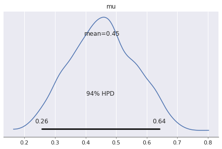
We see the same mean and pretty much the same credibility interval we computed analytically.
It’s kind of an inconvenience not to have a compact representation of the posterior but only samples instead. However this is sometimes all we can hope for in a more complicated, non-conjugate model.
Here’s how we would work with the samples to answer question 2:
print(trace.varnames)
['mu_interval__', 'mu']
trace['mu'].shape
(2000,)
print(f"Probability of a vote for A given the survey result: {trace['mu'].mean()}")
Probability of a vote for A given the survey result: 0.4547869552584988
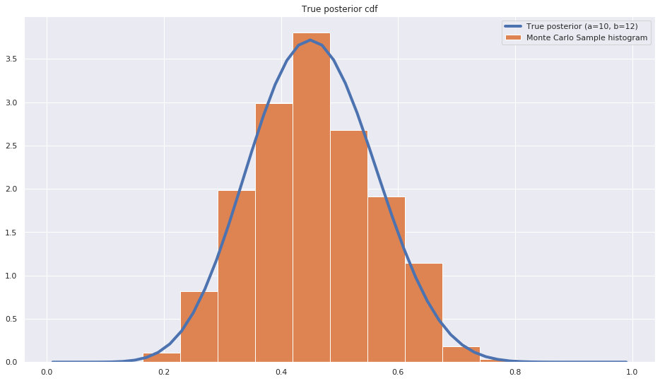
Finally let’s compare the true posterior density to the sample histogram obtained by Monte Carlo sampling
fig = plt.figure(figsize=(16,9))
y = posterior.pdf(x)
plt.plot(x,y, label=f"True posterior (a={observed_votes_for_a+1}, b={num_trials+1-observed_votes_for_a})", lw=4);
plt.hist(trace['mu'], density=True, label="Monte Carlo Sample histogram")
plt.title('True posterior cdf')
plt.legend();
A refresher on the Beta distribution
- Density: $\mathrm{Beta}(\mu, a, b) = \frac{\Gamma(a+b)}{\Gamma(a)\Gamma(b)} \mu^{a-1} (1-\mu)^{b-1}$
- Expected value: $\mathbb{E}[\mu] = \frac{a}{a+b}$
- Variance: $\mathrm{var}= \frac{ab}{(a+b)^2(a+b+1)}$
x = np.linspace(0.01, 0.99)
ab_pairs = [(0.5,0.5), (1, 1), (2,5), (4, 2)]
fig = plt.figure(figsize=(16,9))
for a,b in ab_pairs:
    y = stats.beta.pdf(x, a, b)
    plt.plot(x,y, label=f"(a={a}, b={b})", lw=4)
plt.legend();
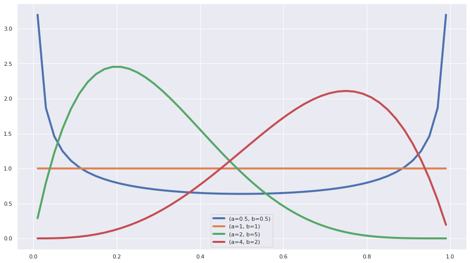
- We see that for values of a and b smaller than 1, the pdf has a U shape.
- For a=1 and b=1 it’s a uniform distribution
- When b is larger than a it’s skewed to the left
- When a is larger than b it’s skewed to the right